Fundamentals of Statistics

Site: EUPATI Open Classroom
Course: Statistics
Book: Fundamentals of Statistics
Printed by: Guest user
Date: Tuesday, 19 March 2024, 8:43 AM

1. Purpose and Fundamentals of Statistics

(This section is organised in the form of a book, please follow the blue arrows to navigate through the book or by following the navigation panel on the right side of the page.)

Data alone is not interesting. It is the interpretation of the data that we are really interested in…
Jason Brownlee – 2018

Statistical methods provide formal accounting for sources of variability in patients’ responses to treatment. The use of statistics allows the clinical researcher to form reasonable and accurate inferences from collected information, and sound decisions in the presence of uncertainty. Statistics are key to preventing errors and bias in medical research.

Hypothesis testing is one of the most important concepts in statistics because it is how you decide if something really happened, or if certain treatments have positive effects or are not different from another treatment. Hypothesis testing is common in statistics as a method of making decisions using data. In other words, testing a hypothesis is trying to determine if, based on statistics, your observations are likely to have really occurred. In short, you want to proof if your data is statistically significant and unlikely to have occurred by chance alone. In essence then, a hypothesis test is a test of significance.

Basics elements of hypothesis testing to be explored:

2. What Is Hypothesis?

A hypothesis is a proposed assumption or set of assumptions for a phenomenon that may or may not be true, and that either

a) asserts something on a provisional basis with a view to guiding scientific investigation (called a working hypothesis); or
b) confirms something as highly probable as opposed to established facts.

For our purposes, we are interested in the hypothesis that asserts something – for example that a new treatment for a disease is better than the existing standard of care treatment. If the new treatment is called ‘B’, and the standard of care treatment is called ‘A’ then the hypothesis states that treatment ‘B’ is better than treatment ‘A’.

Hypothesis testing is the evaluation done by a researcher in order to either confirm or disprove a hypothesis. An existing hypothesis will be taken and tested to see its probability of being true or false.

2.1. Null and Alternative Hypothesis

Setting up and testing hypotheses is an essential part of statistical inference. In each problem considered, the question of interest is simplified into two competing claims or hypotheses, the null hypothesis (H0) and the alternative hypothesis (H1).

The null hypothesis (H0) is formulated to capture our current understanding (the ‘established facts’). The word ‘null’ can be thought of as ‘no change’. A null hypothesis is typically the standard assumption and is defined as the prediction that there is no interaction between variables (a statement that proposes there is no causal relationship, for example, between an investigational medicine and a reduction in symptoms and that outcome measures [even if indicative of a symptom reduction] are due to chance).

The alternative hypothesis (H1) is formulated to capture what we want to show by doing the study. An alternative hypothesis in a clinical trial might be that the new medicine is better than the current standard of treatment against which it is tested.

These two hypotheses should be stated in such a way that they become mutually exclusive. That is, if one is true, the other must be false.

Taking the example from above the hypotheses might be formulated as follows:

  • The null hypothesis (H0): there is no difference between the existing standard of care treatment ‘A’ and the new treatment ‘B’ and any observed differences in outcome measures are due to chance.
  • The alternative hypothesis (H1): the new treatment ‘B' is better than the existing standard of care treatment ‘A’.

2.2. What Is Hypothesis Testing?

Statistical hypothesis testing, also called confirmatory data analysis, is often used to decide whether experimental results contain enough information to cast doubt on established facts. Whenever we want to make claims about whether one set of results are different from another set of results, we must rely on statistical hypothesis tests.

A Hypothesis Test evaluates two mutually exclusive statements, the null hypothesis and the alternative hypothesis, about a population to determine which statement is best supported by data from a sample. Hypothesis tests typically examine a random sample from the population for which statements formulated in the hypotheses should be applicable (valid). The selected samples can range in how representative of the population they are. This is why hypothesis testing on samples can never verify (or disprove) a hypothesis with certainty (i.e. probability in decimal notation = 1) and can only say that a hypothesis has a certain probability to be true or false.

Taking the example from above, H1 stating that a new treatment ‘B’ for a disease is better than the existing standard of care treatment ‘A’, one might presume that scientists would set about proving this hypothesis, but that is not the case. Instead, and somewhat confusingly, this objective is approached indirectly. Rather than trying to prove the B hypothesis, scientific method assumes that in fact A is true – that there is no difference between the standard of care and the new treatment (observed changes are due to chance). The scientists then try to disprove A. This is also known as proving the null hypothesis false. If they can do this – prove that hypothesis A is false, – it follows that B is true, and that the new treatment is better than the standard of care treatment.

An attempt to get behind the reasoning underlying this unusual approach at this point may be to quote Albert Einstein:

“No amount of experimentation can ever prove me right; a single experiment can prove me wrong.”

This seems to suggest that trying to prove the null hypothesis false or wrong is a more rigorous, and achievable, objective than trying to prove the alternative hypothesis is right. Please note that this does NOT properly explain why science adopts this approach, but perhaps it can help us to comprehend and accept a tricky concept more easily.

Statistical tests against the likelihood of chance (or luck) being at the core of observed differences are used in determining what outcomes of a study would lead to a rejection of the null hypothesis and acceptance of the alternative hypothesis. In other words, the result of a hypothesis test is to either ‘reject the null hypothesis in favour of the alternative hypothesis’ with a certain statistically significant probability. As such, the outcome proves the alternative hypothesis. If you fail to reject the null hypothesis, you must conclude that you did not find an effect or difference in your study or that there is ‘not enough evidence to reject the null hypothesis’.

Distinguishing between the null hypothesis and the alternative hypothesis is done with the help of two conceptual types of errors (type I and type II).

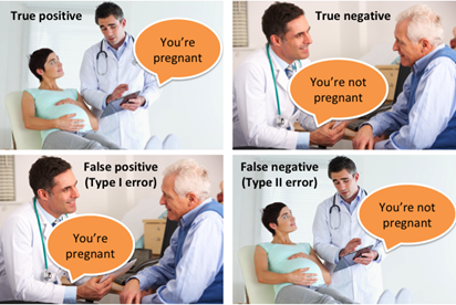
3. Type I and Type II Errors

An experiment testing a hypothesis has two possible outcomes: either H0 is rejected or it is not. Unfortunately, as this is based on a sample and not the entire population, we could be wrong about the true treatment effect. Just by chance, it is possible that this sample reflects a relationship which is not present in the population – this is when type I and type II errors can happen.

All statistical hypothesis tests have a probability of making type I and type II errors. For example, blood tests for a disease will erroneously detect the disease in some proportion of people who don't have it (false positive), and will fail to detect the disease in some proportion of people who do have it (false negative).

Type I - when you falsely assume that you can reject the null hypothesis and that the alternative hypothesis is true. This is also called a false positive result. A type I error (or error of the first kind) is the incorrect rejection of a true null hypothesis. Usually a type I error leads one to conclude that a supposed effect or relationship exists when in fact it doesn't. Examples of type I errors include a test that shows a patient to have a disease when in fact the patient does not have the disease, or an experiment indicating that a medical treatment should cure a disease when in fact it does not. Type I errors cannot be completely avoided, but investigators should decide on an acceptable level of risk of making type I errors when designing clinical trials. A number of statistical methods can be used to control the type I error rate.

Type II error - when you falsely assume you can reject the alternative hypothesis and that the null hypothesis is true. This is also called a false negative result. A type II error (or error of the second kind) is the failure to reject a false null hypothesis. This leads to the conclusion that an effect or relationship doesn't exist when it really does. Examples of type II errors would be a blood test failing to detect the disease it was designed to detect, in a patient who really has the disease; or a clinical trial of a medical treatment concluding that the treatment does not work when in fact it does.


Null hypothesis is true 

Null hypothesis is false 

Reject the null hypothesis 

Type I error
False positive 

Correct outcome
True positive
 

Fail to reject the null hypothesis 

Correct outcome
True negative
 

Type II error
False negative


Example of True positive, true negative, false positive and false negative
In this process of distinguishing between the two hypotheses, specific parametric limits (e.g. how much type I error will be permitted) must also be established. A test's probability of making a type I error is denoted by α (alpha). A test's probability of making a type II error is denoted by β (beta), this number is related to the power or sensitivity of the hypothesis test, denoted by 1 – β. These error rates are traded off against each other: for any given sample set, the effort to reduce one type of error generally results in increasing the other type of error. For a given test, the only way to reduce both error rates is to increase the sample size, and this may not always be feasible.

4. Power of a Statistical Test

A term often used in clinical research is ‘statistical power’. The power of a statistical test is the probability that it will correctly lead to the rejection of a null hypothesis (H0) when it is false– i.e. the ability of the test to detect an effect, if the effect actually exists. Statistical power is inversely related to beta or the probability of making a type II error. In short, power = 1 – β.

In some cases we may not be able to reject the null hypothesis, not because it’s true, but because we do not have sufficient evidence against it. This might be because the experiment is not sufficiently large to reject H0. As such, the power of a test can be described as the probability of not making a type II error (not rejecting the null hypotheses when in fact it false).

Statistical power is affected chiefly by the size of the effect and the size of the sample used to detect it. Bigger effects are easier to detect than smaller effects, while large samples offer greater test sensitivity than small samples

5. Sample Size

In order to have confidence that the trial results are representative, it is critically important to have a ‘sufficient’ number of randomly-selected participants in each trial group. Sample size is the total number of participants included in a trial.

An estimate of the required sample size is needed and must be specified in the study protocol before recruitment starts. It is also necessary to control the probability with which a true effect can be identified as statistically significant.

Too few participants or observations will mean that real effects might not be detected, or they will be detected but at a level that is statistically insignificant (a type II error, which is directly proportional to sample size). It is just as true that it is unacceptable for a medicine to be tested on too many patients. Thus, studies with either too few or too many patients are both methodologically and ethically unjustified. Bear in mind that it is only possible to detect rare side effects in a large sample size and sufficient exposure time, this makes the challenging of estimating sample size complex.

In practice, the sample size used in a study is determined based on:

  1. Magnitude of the expected effect.

  2. Variability in the variables being analysed.

  3. Desired probability that the null hypothesis can correctly be rejected when it is false.

5.1. Sampling Error

In statistics, sampling error may occur when the characteristics of a population are estimated from a subset, or sample, of that population. Since the sample does not include all members of the population, statistics on the sample will differ from parameters under evaluation for the entire population. For example, if one measures the blood pressure of a hundred individuals from a population of one million, the average value for blood pressure won’t be the same as the average value of all one million people.

Since sampling is typically done to determine the characteristics of a population, the difference between the sample and population values is considered a sampling error. The severity of the sampling error can be reduced by increasing the size of the study sample.

6. Significance Level

In everyday language significant means important, but when used in statistics, ‘significant’ means a result has a high probability of being true (not due to chance) and it does not mean (necessarily) that it is highly important. A research finding may be true without being important.

The significance level (or α level) is a threshold that determines whether a study result can be considered statistically significant after performing the planned statistical tests. It is most often set to 5% (or 0.05), although other levels may be used depending on the study. It is the probability of rejecting the null hypothesis when it is true (the probability to commit a type I error). For example, a significance level of 0.05 indicates a 5% risk of concluding that a difference exists when there is no actual difference.


The probability value (p-value) is the likelihood of obtaining an effect at least as large as the one that was observed, assuming that the null hypothesis is true; in other words, the likelihood of the observed effect being caused by some variable other than the one being studied or by chance.

The p-value helps to quantify the proof against the null hypothesis:
The p-value is compared with a pre-defined cut-off for the test (significance level). If it is smaller than this value, the estimated effect is considered to be significant. Often a p-value of 0.05 or 0.01 (written ‘p ≤ 0.05’ or ‘p ≤ 0.01’) are chosen as cut-offs.

This is more easily illustrated by an example:

We have a medicine ‘A’ which decreases blood pressure. We therefore set our null hypothesis as being: ‘Medicine A will NOT decrease blood pressure’. We also decide that the significance level should be 0.05. We run a study using medicine A and observe an average decrease in blood pressure of 20%. Was this due to chance? (null hypothesis true) Or due to the effect of medicine A?`(null hypothesis false). Now we calculate the p-value (the probability) that this result occurred if the null hypothesis was true (the results occurred by chance). The p-value was calculated to be 0.03. Since the p-value (0.03) is less than the significance level we set (0.05) we are able to reject the null hypothesis and conclude that that the measured decrease in blood pressure is likely to be due to the effects of medicine A, rather than being due to chance.

The p-value is compared with a pre-defined cut-off for the test (significance level). If it is smaller than this value, the estimated effect is considered to be significant. Often a p-value of 0.05 or 0.01 (written ‘p < 0.05’ or ‘p< 0.01’) are chosen as cut-offs. These are called the ‘significance levels’ of the experiment.

7. Confidence Interval

The ‘confidence interval’ is used to express the degree of uncertainty associated with a sample statistic. This means that the researcher can only estimate the parameters (i.e. characteristics) of a population, the estimated range being calculated from a given set of sample data.

The confidence interval then is a calculated range of valuesthat is likely to include the population parameter (variable) of interest [in our case, the measure of treatment effect] with a certain degree of confidence. It is often expressed as a % whereby a population parameter lies between an upper and lower set value (the confidence limits).

The likelihood (probability) that the confidence interval will contain the population parameter is called the confidence level. One can calculate a CI for any confidence level, but the most commonly used values are 95% or 99%. A 95% (or 99%) confidence interval will give the range of values (upper and lower) that one can be 95% (or 99%) certain contains the true population mean for the measured effect (the variable of interest) in the sample investigated.

In other words, the confidence interval provides a range for a best guess of the size of the true treatment effect that is plausible given the size of the difference actually observed.

The narrower the confidence interval (upper and lower values), the more precise is our estimate. As a general rule, as the sample size increases, the confidence interval should become narrower. Therefore, with large samples, you can estimate the population mean for the measured effect (the variable of interest) with more precision than you can with smaller samples, so the confidence interval is quite narrow when computed from a large sample. The following figure illustrates this effect.

confidence level

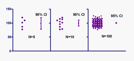
Figure 1: Effect of increased sample size on precision of confidence interval (source https://www.simplypsychology.org/confidence-interval.html)

Confidence intervals (CI) provide different information from what arises from hypothesis tests. Hypothesis testing produces a decision about any observed difference: either that it is ‘statistically significant’ or that it is ‘statistically nonsignificant’. In contrast, confidence intervals provide a range about the observed effect size. This range is constructed in such a way as to determine how likely it is to capture the true – but unknown – effect size.

The following graphs exemplify how the confidence interval can give information on whether or not statistical significance for an observation has been reached, similar to a hypothesis test:

superiority study

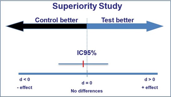
If the confidence interval captures the value reflecting ‘no effect’, this represents a difference that is statistically non- significant (for a 95% confidence interval, this is non-significance at the 5% level).

superiority sutyd 2

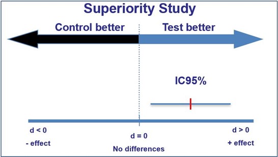
If the confidence interval does not enclose the value reflecting ‘no effect’, this represents a difference that is statistically significant (again, for a 95% confidence interval, this is significance at the 5% level).

In addition to providing an indication of ’statistical significance’, confidence intervals show the largest and smallest effects that are likely, given the observed data, and thus provide additional useful information.