Bias in Clinical Trials
| Site: | EUPATI Open Classroom |
| Course: | Interpretation and Dissemination of Results |
| Book: | Bias in Clinical Trials |
| Printed by: | Guest user |
| Date: | Tuesday, 30 June 2026, 12:58 PM |
1. Where Bias Can Be Introduced
(This section is organised in the form of a book, please follow the blue arrows to navigate through the book or by following the navigation panel on the right side of the page.)Bias can occur at any phase of research, including trial design, data collection, as well as in the process of data analysis and publication. The bias that can occur at different stages during a clinical trial are described in the sections that follow.
1.1. During Participant Recruitment
Selection bias
- If the participant eligibility criteria used in a trial are so stringent that only a small percentage of the intended patient population qualifies. For example, those with better physical condition who would be expected to be able to manage toxic treatments.
- At treatment assignment, the eligibility criteria used to recruit and enrol participants into the treatment arms may be applied differently. This may result in some characteristics being over-expressed in one arm compared to the other. For example, if participants were selected differently according to their age or health status. The treatment outcomes may be stronger in the arm where the participants are younger and in a better shape. Therefore, any difference in outcome between the two treatment arms can no longer be attributed only to the received treatment.
- The use of random participant allocation techniques to two or more treatment arms is key to avoiding this type of bias. Randomisation aims to ensure that the treatment arms are comparable both in terms of known and unknown prognostic factors especially over a large number of participants. Well-performed randomisation will allow the researcher to consider the observed treatment effects (response rate, survival, etc.) to be related to the treatment itself and not due to other factors. The treatment allocation should be independent from researchers’ beliefs and expectations. The optimal way is by using a central randomisation algorithm to distribute characteristics across the treatment arms.
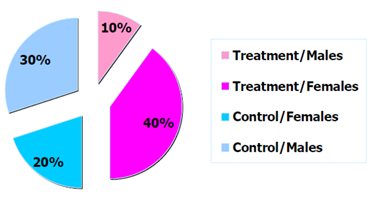
Figure 1: Example distribution of trial participants by arm and sex.
Note that in a trial of limited sample size , there is no guarantee that the randomisation will effectively prevent imbalances in important prognostic factors (age or disease status). In this case, the randomisation can be stratified according to a number of known important prognostic factors. The trial population will be split in groups according to these stratification factors and the randomisation will ensure that the balance between the treatment arms within these strata is maintained.
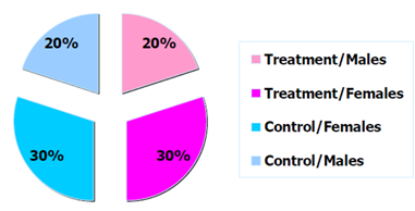
Figure 2: Example distribution of trial participants by arm and sex.
1.2. Information (or Measurement) Bias
This type of bias refers to a systematic error in the measurement of participant characteristics, exposure or treatment outcome, for example:- Participants may be wrongly classified as exposed to being at higher risk of disease when they are not.
- The disease may be reported as progressing when it is stable.
- Inaccuracies in the measurement tool.
- Expectations of trial participants – a participant could be more optimistic because they are assigned to the new treatment group .
- Expectations of the investigators – also called the ‘observer bias’. This occurs when:
- Investigators are very optimistic about the effect of the new treatment and interpret more favourably any clinical signal.
- Investigators monitor the adverse effects of the new treatment more carefully than for the standard treatment.
Blinding the allocated treatment to the participant and/or the investigators may prevent such bias. Blinding is of special interest when the trial outcome is subjective, like the reduction in pain, or when an experimental treatment is being compared to a placebo. However, while a blinded randomised trial is considered the gold standard of clinical trials, blinding may not always be feasible:
-
Treatments may cause specific adverse effects that make them easy to identify.
- Treatments may need different procedures for administration or different treatment schedules.
1.3. During Trial Conduct
- Participants may turn out to be ineligible after randomisation.
- Treatment may have been interrupted or modified but not according to the rules specified in the protocol.
- Disease assessments may have been delayed or not performed at all.
- A participant may decide to stop taking part in the trial, etc.
This can be problematic if not properly accounted for in the analysis. For example, consider the setting of a clinical trial comparing a new experimental treatment to the standard of care. In this trial some participants taking the experimental treatment are too sick to go to the next visit within the allotted time due to side effects. A possible approach would be to include only participants with complete follow-up, so to exclude the sick participants from the analysis. However, by doing so, one selects a sub-group of patients whom, by definition, will present an artificially positive picture of the treatment under trial. This is again an example of selection bias.
One potential solution to this problem is a statistical concept called an intention-to-treat (ITT) analysis. ITT analysis includes every randomised patient whether they received the treatment or not. As such, ITT analyses maintain the balance of patients' baseline characteristics between the different trial arms obtained from the randomisation. ‘Protocol deviations’ such as non-compliance to the assigned treatment (schedule, dosing, etc.) are part of daily practice. Therefore, treatment-effect estimates obtained from ITT analysis are considered to be more representative of the actual benefit of a new treatment
Bias can also happen when measuring the endpoint(s) of interest. For instance, time to disease progression or relapse can be severely affected by the hospital visit schedule. The frequency of disease assessment should be adequate and frequent enough to capture correctly the events that could not be observed by means other than by medical examination at the hospital. The disease assessment schedules should also be the same in both arms.
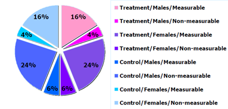
Figure 3: Example of sample distribution by arm and sex.
1.4. During Analysis and Interpretation of Results
- Demographic characteristics (e.g. sex, age).
- Baseline characteristics (e.g. a specific genomic profile).
- Use of concomitant therapy.
- Firstly, sub-group analyses are observational (sub-groups are defined on observed participants’ characteristics) and not based on randomised comparisons. The hindsight bias, also known as the ‘I-knew-it-all-along’-bias, is the
inclination to see events that have already occurred as being more predictable than they were before they took place.
- Secondly, when multiple sub-group analyses are performed, the risk of finding a false positive result (i.e. a type I error) increases with the number of sub-group comparisons. Multiplicity issues are in general related to repeated
looks at the same data set but in different ways until something ‘statistically significant’ emerges. With the wealth of data sometimes obtained, all signals should be considered carefully. Researchers must be cautious about possible over-interpretation.
Techniques exist to protect against multiplicity, but they mostly require stronger evidence for statistical significance to control the overall type I error of the analysis (e.g. the Holm–Bonferroni method and the Hochberg procedure).
- Thirdly, there is a tendency to conduct analyses comparing sub-groups based on information collected while on trial. A typical example is looking at the difference in survival between patients responding (yes/no) to treatment. Participants who are responding to treatment are by definition patients who are able to spend sufficient time on treatment to allow a response. Therefore, again by definition, they may simply represent a sub-group of patients of better prognosis, and may therefore bias the analysis. This is an example of what is often referred to as lead-time bias or guarantee-time bias. One way of dealing with this is using a landmark as a starting point for the time-to-event analysis, and creating the categories based on the participants’ characteristics at the time of this landmark (e.g. did a participant respond at three months, yes/no).